

Other Topics — Machine Learning Interview Questions
Introduction
While training your machine learning model, you often encounter a situation when your model fits the training data exceptionally well but fails to perform well on the testing data, i.e., does not predict the test data accurately. This is where regularization comes into action; Machine learning can handle such situations rightly with regularization. Regularization is a technique to reduce the error by fitting a function appropriately on the given training set and avoid overfitting.
If you are looking for more specific and niche questions geared towards Intermediate and Advanced readers, I recommend you check out some of my other topic specific machine learning question lists here
Article Overview
- What is L1 and L2 Regularization?
- What does the lambda term represent in L1 and L2 Regularization?
- How do L1 and L2 Regularization differ in improving the accuracy of machine learning models?
- Which technique is commonly preferred to boost accuracy rate and why?
What is L1 and L2 Regularization?
There are two common types of regularization known as L1 and L2 regularization. They both work by adding a penalty or shrinkage term called a regularization term to Residual Sum of Squares (RSS).
To understand that, first, let’s look at simple relation for linear regression :
Y≈ β0 + β1X1 + β2X2 + …+ βpXp
Here Y represents the dependent feature or the learned relation, X1, X2, …Xp are the independent features or predictors deciding the value of Y, and β0, β1,…..βn represents the coefficients estimates for different variables or predictors(X), which describes the weights or magnitude attached to the features, respectively.
Now in order to fit a model that accurately predicts the value of Y, we have an optimization function or loss function in simple linear regression, known as the residual sum of squares (RSS).

The model learns with the help of this loss function. The loss function is used to measure the difference between the actual value and the predicted output. The coefficients are chosen in such a way that they minimize the loss function subject to the training data. Suppose there is noise in the training data. In that case, the coefficients will not be able to generalize well to the future data, meaning that the model cannot correctly predict the output or target column for test data. By noise, we mean irrelevant information or randomness in a dataset.
L1 vs L2 Regression Penalty
The L1 and L2 regularization techniques tackle this problem by shrinking or regularizing these learned estimates towards zero by penalizing the magnitude of the coefficients. These penalty terms can be added to any classification problem as well. In a deep learning problem, there are going to be certain optimizers that will be using specific loss functions. To any loss function, we can simply add an L1 or L2 penalty to bring in regularization.
However, both methods differ in the way they assign a penalty to the coefficients.
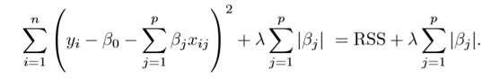
First, let’s check out L1 regularization, also known as Lasso Regression; it modifies the RSS by adding the penalty equivalent to the sum of the absolute value of weight parameters. Mathematically,
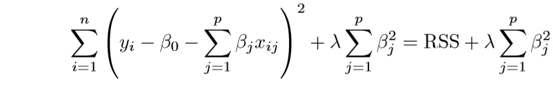
Whereas in L2 regularization, also called Ridge regularization, the penalty term is equivalent to the square of the magnitude of coefficients. The formula is:
What does the lambda term represent in L1 and L2 Regularization?

The free parameter lambda in the penalty term is called a tuning parameter that decides how much we want to penalize our model. In case the values of coefficients get bigger, the loss function will also increase, and our model will not converge, so essentially, we are penalizing higher values of coefficients by adding a penalty here, the lambda parameter acts like a tuning knob and we can control it to minimize the loss function, which means that selecting a good value of is critical.
When λ = 0, the penalty term will have no effect and the coefficients will remain the same as simple linear regression.
When λ = ∞, the impact of the shrinkage penalty grows while the regression coefficient becomes zero.
Else 0 < λ < ∞, for simple linear regression, the regression coefficient will be somewhere between 0 and 1.
How do L1 and L2 regularization differ in improving the accuracy of machine learning models?
The intuitive difference between both techniques is that L2 regression helps us reduce only the overfitting in the model while keeping all the features present in the model. It reduces the complexity of the model by shrinking the coefficients for the least important predictors very close to zero. Whereas L1 regression helps in reducing the problem of overfitting in the model by removing the unnecessary features, it forces the coefficient estimates to be exactly equal to zero.
Sample Calculation for Clarity
To understand it more clearly, we shall consider a simple equation, something like:
y = m1x1 + m2x2 + m3x3 + m4x32 + b
Let’s assume x1 = x2 = x3 = 1 and b = 0
Here we present two weight matrices, i.e., two possible combinations of coefficients.
w1=[1, 0, 0, 0] , y = 1×x1 + 0 + 0 + 0 = 1
w2=[0.26, 0.25, 0.25, 0.25] , y = 0.26×x1 + 0.25×x2 + 0.25×x2 + 0.25×x4 = 1.01
As we can see, after calculating the function value by substituting the weights in our supposed equation, the outputs are nearly equal. In the first case, we get output equal to 1 and in the other case, the output is 1.01. Thus, output wise both the weights are very similar but L1 regularization will prefer the first weight, i.e., w1, whereas L2 regularization chooses the second combination, i.e., w2. The reason behind this selection lies in the penalty terms of each technique.
For the L1 penalty, it tries to minimize the sum of absolute weights. It will pick the weights that have less magnitude. In this case, the sum is 1 for w1 and 1.01 for w2.
On the other hand, the L2 penalty minimizes the sum of squared weights. So, the sum of squares for w1 is going to be 1, but the sum of squares for w2 is going to be much less than 1. In this way, both techniques will favor the weights that help them minimize their penalty term.
Implications of Using Each Technique
Now, if we observe the first set of coefficients that L1 chooses, we only have a single weight equal to 1, and the rest of the weights are zero. It is basically saying that all other features are not important, and we are selecting only one feature; this is what feature selection is. L1 regularization automatically removes the unwanted features. This is helpful when the number of feature points are large in number. However, L2 regularization provides a robust model; it takes all the features into consideration but gives moderate importance to each feature, which means the final model will include all independent variables, also known as predictors.
Which technique is commonly preferred to boost the model’s accuracy rate and why?
One cannot really draw a conclusion as to which technique provides a better accuracy rate as it depends on several factors. Although L2 is majorly used to prevent overfitting, it is not very useful in the case of high-dimensional data, as it will pose computational challenges. It is preferred when many features are highly correlated with the target. For modeling cases where the features are in millions, L1 regularization is the desired technique as it provides sparse solutions. A sparse model is a great property to have when dealing with exorbitantly high features. Eventually, it depends on the real-world problem at hand and our model objective.


