

Introduction
Feature extraction and feature selection are two critical processes in machine learning. While they may be confused to mean the same thing, they are slightly different. The difference between both terms will be discussed momentarily. Suffice it to say that both are feature reduction techniques aimed at improving the machine learning model’s performance.
Data comes in different sizes. Sometimes, with a few features and other times, with thousands of features. While working with huge data is the perfect recipe for building a robust model, the number of features may increase to a certain stage that some of them become noise. This causes the performance of the model to drop – a phenomenon called the curse of dimensionality.
Feature reduction helps to:
- Speed up the training time of the model
- Improve the accuracy of the model trained on a noisy dataset and
- Enhance data visualization
This article will walk you through how to perform both feature extraction and feature selection in machine learning. You will also discover how to use the different methods for each of the processes. For better understanding, we will build a machine learning model that uses both feature extraction and feature extraction techniques. The dataset used is obtained from the dataset and can be downloaded here.
By the end of this article, you will understand:
- The difference between feature extraction and feature selection.
- How to use both methods in machine learning.
- The appropriate situation to implement each of the methods.
Article Overview:
- Feature Extraction: What is it?
- Building a Baseline Logistic Regression Model
- Principal Component Analysis (PCA) for Feature Extraction
- Linear Discriminant Analysis (LDA) for Feature Extraction
- Isomap for Feature Extraction
- Locally Linear Embedding (LLE) for Feature Extraction
- Feature Selection: What is it?
- Random Forest for Feature Selection
- SelectFromModel for Feature Selection
We begin with feature extraction. So without further ado, let’s jump into it.
Feature Extraction: What it is?
Feature extraction reduces the number of features in a dataset by creating a new set of features whose length is shorter than the initial one. Putting it differently, it is a way of merging features to smaller ones while still largely maintaining the intrinsic properties of the initial features. What’s important here is that the new features should summarize the original features without losing much information. This is an important step, especially when there are many features. In addition, feature extraction helps to reduce the data to a manageable group where preprocessing becomes easier.
We’d discuss the process of feature extraction using a worked example. To get started, we select a dataset to build the machine learning model.
The Breast Cancer Dataset

We will use the breast cancer dataset for this illustration. The data has 569 samples and 31 numeric columns. The dependent variable (or label) is a binary classification showing where a person has breast cancer or not. Some of the independent variables (or features) are:
- Radius: The mean of distances from center to points on the perimeter.
- Texture: The standard deviation of the grey scale values
- Perimeter
- Area
- Smoothness
- Compactness
- Concavity
- Concave points, and so on.
To be clear, the dataset has 30 features. This dataset of one scikit-learn default dataset and thus, it will be imported from the library.
Building the Baseline Model – Logistic Regression
In this step, we build a simple baseline model without feature reduction. First, we import the necessary libraries.
#import the necessary libraries
import numpy as np
import pandas as pd
import matplotlib.pyplot as plt
import seaborn as sns
from time import time
from sklearn.datasets import load_breast_cancer
Next, we call the cancer dataset from the package and save it in a variable called cancer_dict.
cancer_dict = load_breast_cancer()By default, the dataset is a dictionary that contains the feature data, label data, feature name, label name, a description of the data and the file name. To confirm that, we print the keys of the dictionary.
cancer_dict.keys()Output:
dict_keys(['data', 'target', 'frame', 'target_names', 'DESCR', 'feature_names', 'filename'])Next, we split the data into features and columns and then convert them into a dataframe.
#define the feature and labels in the data
data = cancer_dict.data
columns = cancer_dict.feature_names

X = pd.DataFrame(data, columns=columns)
y = pd.Series(cancer_dict.target, name='target')

#merge the X and y data
df = pd.concat([X, y], axis=1)
df.sample(10)
Output:
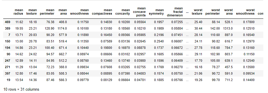
As seen, the dataset has 32 columns; 30 features (X)and 1 label (y).To ensure the model performs well, the dataset needs to be scaled. The StandardScaler class was used to scale the data such that it follows a normal distribution curve.
Of course, the necessary libraries were imported.
from sklearn.preprocessing import StandardScaler
from sklearn.model_selection import train_test_split
from sklearn.linear_model import LogisticRegression
from sklearn.metrics import accuracy_score, recall_score, precision_score

#scale the data
scaler = StandardScaler()
X_scaled = scaler.fit_transform(X)
Now, let’s create a function that receives the X and Y data, applies a machine learning model and returns the performance metrics of the model. The data was split into train and test using a 70:30 splitting ratio and a logistic regression model was applied on the data. By the way, logistic regression is a fantastic algorithm for binary classification problems such as ours.
The code snippet for the function is shown below.
def apply_model(X, y):
    '''
    This function receives the X and y dataset set, splits into train and test,
    applies a Logistic Regression algorithm on the train data, make prediction after training,
    and returns the recall
    '''

    #split the data
    X_train, X_test, y_train, y_test = train_test_split(X, y, random_state=1, test_size=0.3)

    #apply the Logistic Regression algorithm on the data
    model = LogisticRegression()
    model.fit(X_train, y_train)

    #make prediction
    y_pred = model.predict(X_test)

    #compute the metrics
    accuracy = accuracy_score(y_test, y_pred)
    recall = recall_score(y_test, y_pred)
    precision = precision_score(y_test, y_pred)

    return(f"Accuracy score: {accuracy}",
           f"Recall score: {recall}",
           f"Precision score: {precision}"
          )
We can call the function on the dataset without any feature reduction.
%time apply_model(X_scaled, y)Output:
Wall time: 64 ms
(‘Accuracy score: 0.9707602339181286’,
‘Recall score: 0.9722222222222222’,
‘Precision score: 0.9813084112149533’)
Also, notice the time it took for the computation to be complete. Now, let’s discuss some feature extraction techniques that can be applied to the data.
Feature Extraction with Principal Component Analysis (PCA)

Principal Component Analysis is one of the most popular feature reduction techniques. It finds a way of reducing the number of features by finding a smaller combination of features that best summarises the initial feature. PCA basically uses metrics such as variance and reconstruction error when performing this transformation. It attempted to maximize variance and minimize reconstruction error. PCA projects the initial dataset to a set of orthogonal axes. Datapoints that are highly correlated are clustered together in the new axes. These axes are then ranked based on their order of importance.
PCA is classified as an unsupervised learning algorithm and thus, does not require the labels of the data. In fact, PCA can be used to reduce the dataset dimension to 1, where the classification is done already. Note, however, that since it is an unsupervised learning model, there could be misclassification in some situations.
For the breast cancer dataset, PCA will be applied to reduce the dataset features to only two – from 30 to 2. After this transformation, the logistic regression algorithm can be used for classification.
Let’s use PCA to create a new dataset with just 2 columns.
from sklearn.decomposition import PCA

pca = PCA(n_components=2)

#apply PCA to transform the features to 2
X_pca = pca.fit_transform(X_scaled)

#create the new dataframe
df_pca = pd.concat([pd.DataFrame(X_pca), y], axis=1)
This is what the dataset looks like now.
df_pca.head()Output:
| 0 | 1 | target | |
| 0 | 9.192836826 | 1.948583071 | 0 |
| 1 | 2.387801796 | -3.768171742 | 0 |
| 2 | 5.73389628 | -1.075173797 | 0 |
| 3 | 7.122953198 | 10.27558912 | 0 |
| 4 | 3.935302074 | -1.948071568 | 0 |
We can visualize the data points in a 2D scatter plot.
#visualize the dataset
sns.scatterplot(df_pca.iloc[:, 0], df_pca.iloc[:, 1], hue=df_pca['target'])
Finally, we apply the machine learning model for prediction using the already created function.
%time apply_model(X_scaled, y)Output:
Wall time: 24 ms
(‘Accuracy score: 0.9415204678362573’,
‘Recall score: 0.9537037037037037’,
‘Precision score: 0.9537037037037037’)
Notice, the process was done in a shorter time and the results were still outstanding.
Feature Extraction with Linear Discriminant Analysis (LDA)

LDA reduces the dimension by maximizing the separability among each feature. It works by creating a new feature (you could see it as a line) and projecting all the other features on that line. During transformation, LDA attempts to maximize the distance between the mean of every feature. Also, the scattered amongst the data points need to be minimized. By doing these, there would be a minimal overlap of data points on the new axis. Less overlap means there will be minimal misclassification, and by extension, means there will be better classification results.
LDA is a supervised learning classifier which means it requires both the features and the labels (or X and y).
In the example below, we would apply LDA on the data to reduce the dataset to just 1 feature.
#import the LDA class
from sklearn.discriminant_analysis import LinearDiscriminantAnalysis

#instantiate the LDA class and setting the number of components to 1
lda = LinearDiscriminantAnalysis(n_components=1)

#apply the LDA class
lda.fit(X_scaled, y)
X_lda = lda.transform(X_scaled)

#get the resulting data
df_lda = pd.concat([pd.DataFrame(X_lda), y], axis=1)
We can visualize how LDA has successfully compressed the dataset to just one feature.

As seen, the data has just one feature and has successfully classified the target as either 0 or 1. So, let’s check the performance of LDA feature reduction.
%time apply_model(X_scaled, y)Output:
Wall time: 16 ms
(‘Accuracy score: 0.9649122807017544’,
‘Recall score: 0.9907407407407407’,
‘Precision score: 0.9553571428571429’)
Notice the results were almost perfect. And it was done at 16 milliseconds. Pretty fast!
Feature Extraction with Isomap
PCA and LDA methods considered above reduce features by finding the relationship between features after projecting them on an orthogonal plane. LLE (explored in the next section below) is quite different in the sense that it does not use linear relationships but also accommodates non-linear relationships in the features. Isomap works by using a type of learning called manifold learning.
Manifold learning summarises the data to a smaller number of features. This time however, the generalization is made to be such that it is sensitive to any form of non-linear structure in the dataset.
Isomap creates a lower-dimensional embedding of the data while maintaining the geodesic (or mean) distance between all points in the dataset. Let’s see how Isomap works in Python.
#import Isomap
from sklearn.manifold import Isomap

#apply Isomap on the data
iso = Isomap(n_components=2)
X_iso = iso.fit_transform(X_scaled)

#create the new dataset
df_iso = pd.concat([pd.DataFrame(X_iso), y], axis=1)
Next, we visualize the new data.
sns.scatterplot(df_iso.iloc[:, 0], df_iso.iloc[:, 1], hue=df_iso['target'])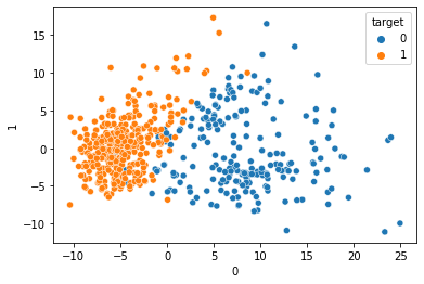
Finally, the dataset is passed to the apply_model function to see how it performs
%time apply_model(X_scaled, y)Output:
Wall time: 393 ms
(‘Accuracy score: 0.9590643274853801’,
‘Recall score: 0.9722222222222222’,
‘Precision score: 0.963302752293578’)
One thing to observe here is that the Isomap reduction technique has an incredibly great performance. However, it takes longer to train. These are some of the tradeoffs that are required in machine learning. Nevertheless, if you care about the result and could spare extra computational time, Isomap is a great option for dimensionality reduction.
Feature Extraction with Locally Linear Embedding (LLE)

Locally Linear Embedding is another non-linear feature reduction technique that utilizes manifold learning as well. According to the official documentation of sci-kit learn, locally linear embedding attempts to find a lower-dimensional projection that preserves the distance between the local neighborhoods. We can run the LLE algorithm on the dataset and see how well it performs.
#import LLE
from sklearn.manifold import LocallyLinearEmbedding

#create an instance of the class
lle = LocallyLinearEmbedding(n_components=2)
X_lle = lle.fit_transform(X_scaled)

#create the new dataset
df_lle = pd.concat([pd.DataFrame(X_lle), y], axis=1)
Next, we perform the visualization.

FInally, we call the apply_model() function on the new dataset.
%time apply_model(X_scaled, y)Output:
Wall time: 19 ms
(‘Accuracy score: 0.6374269005847953’,
‘Recall score: 1.0’,
‘Precision score: 0.6352941176470588’)
Apparently, the LLE technique did not do so well in classifying the data, even though it was computed at a faster time than Isomap. It is not to say that LLE is not generally a good technique; it just may not be good for this data. That is why it is advisable to try out as many models as possible on your dataset and select the data. A model that works well on one dataset might not work well on another.
One thing to point out is that while LLE and Isomap work using the same foundational principle, LLE runs faster than Isomap.
And this will be a wrap on this feature extraction technique. Let’s now turn our attention to feature selection.
Feature Selection: What it is?
Feature selection describes techniques that completely eliminates features that are less important in the data. As earlier mentioned, it is a rule of thumb that more features allow the machine learning model to learn better. However, as the feature increases to some point, the model will begin to find it difficult to utilize all the features for the prediction. Many of the extra features become noise, and this adversely impacts the performance of the model. This is why feature selection is critical. When you have a dataset with lots of features, you necessarily do not need all the features for optimum performance. You can decide to filter only the most important features and leave out those that are less important for the modelling.
Let’s see how to apply feature selection on the breast cancer data.
Feature Selection using Random Forest
Random forest is an ensemble of decision trees that can be used to rank the importance of the features in the data. Having known this, the less important ones can be discarded before feeding the data in a machine learning model.
To do this in Python, we begin by importing the RandomForestClassifier class
#import the random forest class
from sklearn.ensemble import RandomForestClassifier
Afterwards, we build a machine learning pipeline that splits the data into train and test data. The random forest classifier will then be applied to the training dataset only and finally be used to make predictions. The metrics used for model evaluation were accuracy, recall, and precision.
The code snippet for this process is shown below.
#split the model into train and test data
X_train, X_test, y_train, y_test = train_test_split(X_scaled, y, random_state=1, test_size=0.3)

#apply the dataset on the model
rfc = RandomForestClassifier()
rfc.fit(X_train, y_train)

#make prediction
y_pred = rfc.predict(X_test)

#evaluate the model
accuracy = accuracy_score(y_test, y_pred)
recall = recall_score(y_test, y_pred)
precision = precision_score(y_test, y_pred)

#print the result
print(f"Accuracy score: {accuracy}",
       f"Recall score: {recall}",
       f"Precision score: {precision}"
      )
Output:
Accuracy score: 0.9532163742690059
Recall score: 0.9814814814814815
Precision score: 0.9464285714285714
It appears that the random forest model does quite well. But beyond making predictions, the random forest model classifier can be used to determine the most important features.
These features are ranked and can be found using the feature_importances_ attribute of the random forest object.
The code below converts the list of ranked feature importance and converts it to a pandas series.
feature_importance = pd.Series(rfc.feature_importances_, index= X.columns)
feature_importance.sort_values(ascending=False)
Output:
worst concave points 0.169392
worst perimeter 0.153736
worst area 0.097411
mean area 0.074427
mean perimeter 0.072978
mean concave points 0.072780
worst radius 0.066819
mean concavity 0.048515
mean radius 0.038357
worst concavity 0.035495
area error 0.027703
worst texture 0.017105
mean texture 0.016450
mean compactness 0.016190
concave points error 0.009904
worst smoothness 0.009661
perimeter error 0.008822
radius error 0.008504
worst compactness 0.007722
worst symmetry 0.007657
concavity error 0.005393
mean smoothness 0.004601
compactness error 0.004481
smoothness error 0.004240
fractal dimension error 0.004091
mean symmetry 0.003839
mean fractal dimension 0.003825
worst fractal dimension 0.003702
symmetry error 0.003229
texture error 0.002979
The output above is a list of feature importance ranked from highest to lowest. We can make a visualization for the first 10.
feature_importance.nlargest(10).plot(kind='barh')Output:
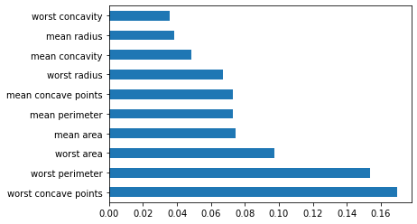
As seen, here are the 10 most important features in the dataset. You can drop the other ones and apply your machine learning model using these 10 features alone.
Feature Selection using SelectFromModel
SelectFromModel is a class in sci-kit learn that can be used for feature selection. This method uses a machine learning model for fitting then determines the less important features by cutting off features that do not meet some calculated threshold.
In our example, the Logistic Regression model is used alongside the SelectFromModel algorithm. One thing to note, however, is that the penalty must be set to L1. L1 regularization, also called Lasso, reduces the number of features by adding an L1 penalty to the absolute value of the magnitude of the coefficients.
Now, let’s apply SelectFromModel on the breast cancer dataset using the LogisticRegression algorithm.
#import the necessary library
from sklearn.feature_selection import SelectFromModel

#instantiate the class using the L1 regularizer and a liblinear solver
selection = SelectFromModel(LogisticRegression(C=1, penalty='l1', solver='liblinear'))
selection.fit(X_train, y_train)
The get_support() method is used to return the features of the SelectFromModel. It returns a boolean for each feature. True means the feature should be kept, while false implies that the feature should be discarded.
Let’s check the number of features that should be kept.
len([x for x in selection.get_support() if x==True])Output:
15
15 features were kept, while 15 were discarded. We can print the selected features using the code below.
X.columns[(selection.get_support())].to_list()Output:
[‘mean concavity’,
‘mean concave points’,
‘mean fractal dimension’,
‘radius error’,
‘smoothness error’,
‘compactness error’,
‘fractal dimension error’,
‘worst radius’,
‘worst texture’,
‘worst perimeter’,
‘worst area’,
‘worst smoothness’,
‘worst concavity’,
‘worst concave points’,
‘worst symmetry’]
You’d notice a huge intersection between the results from this method and the random forest technique.
Wrapping up
In this article, you have learned the difference between feature extraction and feature selection. To recap, they are both feature reduction techniques, but feature extraction is used to ‘compress’ the number of features, whereas feature selection is used to completely eliminate less important features.
We went ahead to apply several feature extraction and feature selection techniques using the breast cancer dataset. If you have any questions, feel free to leave them in the comment section. Thanks for reading!
Further Readings
For Beginners
Exploratory Data Analysis for Beginners
Barebones Linear Algebra for Machine Learning (Only the Essentials)
For Intermediate Readers
Comprehensive Guide on Feature Selection (Requires Statistics + Linear Algebra Knowledge)


")

