

Introduction
Linear algebra is the backbone of machine learning and is critical for learners to have a solid understanding of the concepts before jumping into the core of machine learning. First, let’s take some time to understand why linear algebra before getting into the crux of linear algebra.
Article Overview
- Why Linear Algebra?
- What is the Transpose of a Matrix?
- Different Forms of Matrices
- Special Matrices
- Norms of Matrices
- Multiplications of Matrices and Vectors
- Linear Independence and the Rank of a Matrix
- How to do Matrix Inversion?
- Trace and Determinant of a Matrix
- Eigenvalues and Eigenvectors
- What is Singular Value Decomposition (SVD)?
Why Linear Algebra?
It’s simple. Linear algebra provides a compact way of representing equations and performing some operations on them. For example, the two equations:
\begin{aligned} &4 x+7 y=15 \\ &3 x-5 y=-1 \end{aligned}Can be written in the form
A x=bWhere
A=\left[\begin{array}{cc} 4 & 7 \\ 3 & -5 \end{array}\right] \text { and } b=\begin{array}{cc} 15 \\ -1 \end{array}We represent our system of equations with two matrices. A matrix that has only one row or only one column it is called a vector. Therefore, our b matrix is a vector.
What is the Transpose of a Matrix?
The transpose of the matrix is simply the result of the matrix when the row is changed to the column and vice versa. In other words, the transpose of a matrix with i rows and j columns results in a matrix with j rows and i columns. The statement can be written mathematically as:
A_{i j}^{T}=A_{j i}Given this definition, the following mathematical expressions are true.
\begin{gathered} \left(A^{T}\right)^{T}=A \\ (A B)^{T}=B^{T} A^{T} \\ (A+B)^{T}=A^{T}+B^{T} \end{gathered}Different Forms of Matrices
- Square matrix: A square matrix is any matrix where the number of rows is equal to the number of columns.
- Symmetric matrix: A matrix is symmetric if the transpose of the matrix is equal to the matrix itself. Mathematically,
- Anti-symmetric matrix: A matrix is asymmetric if the transpose of the matrix is equal to the negative of the matrix. Mathematically,
It is important to note that symmetric and asymmetric matrices are always square matrices. As a rule of thumb, every matrix can be rewritten as the sum of symmetric and anti-symmetric matrices.
Special Matrices
- Identity matrix: A matrix where the diagonal is filled with ones and zeroes everywhere else.
- Diagonal matrix: This is a type of matrix where all non-diagonal matrices are zero. Thus, an identity matrix is a type of diagonal matrix.
Norms of Matrices
To define succinctly, the norm of a vector is the measure of its ‘length’ or magnitude. The norm of a function generally to satisfies the following properties:
- Non-negativity: The vector is a positive real number
- Definiteness: The vector is equal to 0 if and only if all the elements of the vector are equal to zero.
- Homogeneity: The vector that has some scalar multiplier is equal to the vector multiplied by the absolute value of the scalar. Written mathematically, it is:
Where f(t x) is the function and t is the scalar.
- Triangle inequality: The function of the sum of more than one element is always less than or equal to the sum of the function with each element. Mathematically,
What Types of Norms are Used in Machine Learning?
Norms are calculated using many different methods. The common ones used in machine learning are:
- L2 norm: This is simply the square root of the sum of the square of each element.
Given a position A and B in a dimensional space, the L2 norm is the shortest distance between the vectors.
- L1 norm: This is the sum of the absolute value of each element of the function.
Given a position A and B in a dimensional space, the L1 norm is the Manhattan distance between the two points.
- L infinity norm: This is the maximum absolute value of the elements of the vector.
There are tradeoffs between the use of L1 and L2. L1 is great since it avoids the equidistance situation between different points. L2 on the other hand, allows the problem to be easily optimized.

For a more in-depth explanation of the difference between L1 and L2 click here.
Multiplications of Matrices and Vectors
Matrix multiplication
The product of two matrices A and B is given by c, where
C_{i j}=\sum A_{i k} B_{k j}Vector multiplication
The multiplication of a vector is done in two ways. The first way is through the inner dot product:
x y^{T}=\left[\begin{array}{lll} x_{1} & x_{2} & x_{3} \end{array}\right]\left[\begin{array}{l} y_{1} \\ y_{2} \\ y_{3} \end{array}\right]=\sum_{i=1}^{3} x_{i} y_{i}Geometrically, the dot product can be represented as
x \cdot y=|x||y| \cos \thetaWhere \theta is the angle between x and y. The inner products give an insight into how two vectors are correlated. For instance, if x\cdot y > 0, it means that when x increases, y increases. Conversely, if x\cdot y < 0, it means that when x increases, y decreases. Finally, if x\cdot y = 0, they are not related at all.
The second way to multiply vectors is with the outer product:
The outer product of two vectors (denoted as x \otimes y) is given by
x \otimes y=\left[\begin{array}{l} x_{1} \\ x_{2} \\ x_{3} \end{array}\right]\left[\begin{array}{lll} y_{1} & y_{2} & y_{3} \end{array}\right]=\left[\begin{array}{lll} x_{1} y_{1} & x_{1} y_{2} & x_{1} y_{3} \\ x_{2} y_{1} & x_{2} y_{2} & x_{2} y_{3} \\ x_{3} y_{1} & x_{3} y_{2} & x_{3} y_{3} \end{array}\right]Linear Independence and the Rank of a Matrix
A matrix is said to be linearly independent if no row or column can be represented as the scalar multiplication of another row and column. Otherwise, it is linear dependent. For example, a matrix with rows 1, 2, 3 and 2, 4, 6 would be linearly dependent since the second row is 2 multiplied by the first row.
The row/column rank of a matrix is the size of the largest subset of rows/columns that constitute a linearly independent set. Simply put, it is the number of unique rows or columns. A matrix where all rows and columns are independent is a full rank matrix.
Let’s see some examples.
Examples
1. What is the rank of this matrix?
\left[\begin{array}{ll} 1 & 2 \\ 2 & 4 \\ 3 & 6 \end{array}\right]Row rank: First, the matrix has 3 rows. The second row is the scalar multiple of the first and the third row is a scalar multiple of the first as well. In other words, there is 1 unique row.
Column rank: First, the matrix has 2 columns. The second row is a scalar multiple of the first. Since there is one unique column rank is 1
Therefore, Rank = 1.
Note: In a situation where the column rank and row rank are different, the rank of the matrix is the rank with the lowest value. So, say the column rank was 3 and the row rank was 1, the rank of the matrix will be 1.
2. What is the rank of this matrix?
\left[\begin{array}{lll} 1 & 0 & 2 \\ 2 & 1 & 0 \\ 3 & 2 & 1 \end{array}\right]Looking at the above matrix, there is no unique row or column. All rows and columns seem to be completely independent of each other. Thus, this is a full rank matrix. Rank = 3.
How to do Matrix Inversion?
The inverse of a square matrix A is denoted by A^{-1} and is a unique matrix that satisfies the following condition.
A^{-1} A=I=A A^{-1}If the inverse of a square matrix does not exist, then the matrix is called a singular matrix or non-invertible matrix.
For a non-square matrix, the inverse denoted by A^{+} is given by
A^{+}=\left(A^{T} A\right)^{-1} A^{T}Where A^{T} is the transpose of the matrix. The inverse of a non-square matrix is called a pseudo matrix.
Trace and Determinant of a Matrix
The trace of the matrix is simply the sum of the diagonal element in that matrix. It is especially useful when computing the norms and Eigenvalues of matrices. We will discuss how to do this momentarily.
The determinant of a matrix, A is denoted by |A| and is given by
\operatorname{det}(A)=\sum_{j=1}^{d}(-1)^{i+j} a_{i j} M_{i j}Where M_{i j} is the determinant of matrix A without the row i and column j.
How to find the Determinant of a 2 x 2 Matrix?
The determinant of a 2 by 2 matrix,
\left[\begin{array}{ll} a & b \\ c & d \end{array}\right]is given by (ad - bc)
What are the Properties of a Determinant?
The determinant of the matrix has some special properties. They include:
- The determinant of a matrix is equal to the determinant of the transpose of the matrix
- Determinant of the product of two matrices is equal to the determinant of each of the matrices and finding their product.
- The determinant of a matrix is zero if and only if the matrix is not invertible. In other words, the matrix is a not full rank matrix.
Eigenvalues and Eigenvectors
Eigenvalues and eigenvectors are critical transformations of a matrix. This concept helps us convert a matrix to a vector. It says that if we have a matrix A, we can get a vector x scaled by a parameter \lambda by multiplying the vector x by A. Mathematically,
A x=\lambda xWhere A is the matrix, X is the vector that is not equal to 0, and \lambda is the multiplying parameter or scalar.
The above equation can be rewritten as (A-\lambda I) x=0. For this to be true, it means (A-\lambda I) must be singular or Z=|A-\lambda I|=0.
Steps to Calculating the Eigenvalues and Eigenvectors
Step 1: Compute the determinant of A-\lambda I. This results in a polynomial of degree d
Step 2: Find the root of the polynomial by equating it to 0. The roots of the polynomial are the eigenvalues.
Step 3: Solve for x in the equation (A-\lambda I)x. x is the eigenvectors.
Let’s take an example.
Example
Find the eigenvalues and eigenvectors of the matrix:
\left[\begin{array}{cc} 1 & 2 \\ 3 & -4 \end{array}\right]Solution
Step 1: Compute |A-\lambda I|
|A-\lambda I| \text { ie }\left[\begin{array}{cc} 1 & 2 \\ 3 & -4 \end{array}\right]-\left[\begin{array}{cc} \lambda & 0 \\ 0 & -\lambda \end{array}\right]=0Step 2: Compute the determinant and equate it to zero
\begin{aligned} &\text { Determinant of }\left[\begin{array}{cc} 1 & 2 \\ 3 & -4 \end{array}\right]-\left[\begin{array}{cc} \lambda & 0 \\ 0 & -\lambda \end{array}\right]=0 \\[15pt] &\left|\begin{array}{cc} 1-\lambda & 2 \\ 3 & -4-\lambda \end{array}\right|=0 \\[15pt] &(1-\lambda)(-4-\lambda)-6=0 \end{aligned}Solving the quadratic equation, \lambda = -5 and \lambda = 2
Step 3: Solve A x=\lambda x, \text { where } x=\left[\begin{array}{l} x_{1} \\ x_{2} \end{array}\right] \text { since the matrix is of size } A \text { . }
That is,
\left[\begin{array}{cc} 1 & 2 \\ 3 & -4 \end{array}\right] \cdot\left[\begin{array}{l} x_{1} \\ x_{2} \end{array}\right]=\lambda \cdot\left[\begin{array}{l} x_{1} \\ x_{2} \end{array}\right]Carrying out the multiplication leads to a simultaneous equation
\begin{array}{r} x_{1}+2 x_{2}=\lambda x_{1} \\ 3 x_{1}-4 x_{2}=\lambda x_{2} \end{array}For \lambda = -5, solving the equation gives x_{1} = 1, -3 and for \lambda = 2, solving the equation gives x_{2} = 2, -1.
Therefore, the eigenvectors are \left[\begin{array}{c} 1 \\ -3 \end{array}\right] \text { and }\left[\begin{array}{c} 2 \\ -1 \end{array}\right]
What is Singular Value Decomposition (SVD)?
Single value decomposition is a method to find the eigenvalues and eigenvectors of a covariance matrix. Given a matrix X, the singular value decomposition matrix is given by:
X=U \Sigma V^{T} \begin{aligned} & \text{Where } \mathrm{U}\text{ is a unitary matrix, i.e, }U * U^{T}=I \\ & \Sigma \text{ is a diagonal matrix} \\ & V_{d * d}\text{ is a unitary matrix, ie }V * V^{T}=I \end{aligned}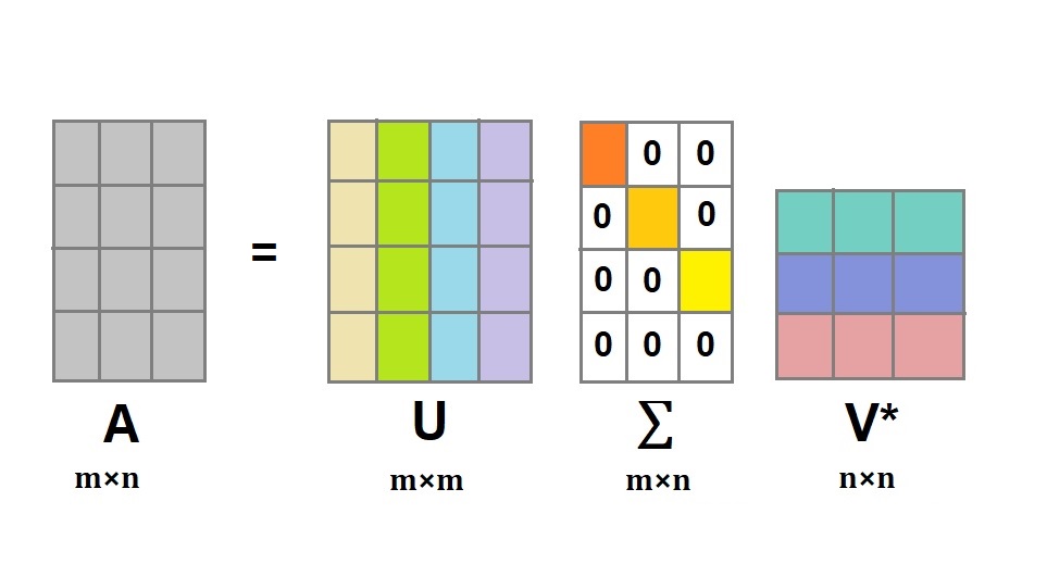
To calculate the covariance of a matrix, we first center the matrix. Centering means finding the average of the elements of each row then subtracting each element by that average. Finally, we divide the value found by the number of rows present. It is just like the conventional way of finding the average number in a list.
The covariance shows the relationship between features (or rows) of the matrix. After finding the covariance, it is convectional to scale them. Our matrix can be scaled in two ways:
- Standardization: This is when the values are scaled between 0 and 1.
- Normalization: This is the scaling of the values between -1 and 1. It is important when you do not want to lose track of negative numbers.
Singular Value Decomposition for Dimensionality Reduction in Machine Learning
Singular Value Decomposition provides a way of reducing the dimensionality of a dataset. It finds the best plane/axis that data points can be projected on with minimum sum of squares projection errors. For instance, it could represent a data point in a 2-dimensional plane to a point along a line with a minimum reconstruction error. In other words, the distance between its initial position in the 2-dimensional space and the position on the line should be minimum.
So, how do you determine the best axis as well as the position on a given axis?
The singular vector provides the axis upon which the points should be projected. On the other hand, the singular value provides the variance or the spread in the projected axis. A high singular value indicates that the data points should be spread well along that axis whereas a low singular value indicates that they should compact along that axis. U \Sigma is used to determine the position of the coordinates in the projected axis.
To find the dimension reduction with minimum reconstruction error, the smallest singular values are set to zero. Simply put, the smallest column values in U is set to zero, the smallest diagonal in \Sigma is set to zero and the smallest row in V^{T} is set to zero.
The computation of U \Sigma V^{T} after this would result in a matrix that is close to the initial matrix, however, the matrix is smaller. This is how dimensionality reduction is done with SVD.


")
