

Introduction
When a deep neural network ends up going through a training batch, where it propagates the inputs through the layers, it needs a mechanism to decide how it will use the predicted results against the known values to adjust the parameters of the neural network. These parameters are commonly known as the weights and biases of the nodes within the hidden layers.
This above-mentioned mechanism is where the optimizers kick in. Optimizers are the algorithms deciding how the learning parameters are adjusted. These optimizers, along with the loss functions, are the backbone of all deep neural networks.
Throughout this guide, we’ll go through a detailed explanation of how the optimizers work and the different types of optimizers that Keras provides us, along with instantiation examples. Moreover, we’ll also be taking a look at the situations where certain optimizers work better than others.
Article Overview
- How Do Optimizers Work?
- How To Use Optimizers in Keras?
- SGD Optimizer
- Adagrad Optimizer
- RMS Optimizer
- Adadelta Optimizer
- Adam Optimizer
- Summary
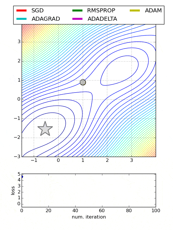
How Do Optimizers Work?
To get a solid intuition, imagine hiking down a mountain where your eventual aim is to reach the lowest point of the mountain, however, you cannot use your eyes to guide you. How will you achieve this? Well, you can simply follow the path that leads you downwards (has a decreasing slope) and eventually, you’ll reach the lowest point there is, right?
Turns out, it’s exactly what an optimizer does. While the slope of a mountain refers to the loss or cost function of a neural network, the optimizer guides and helps the network achieve the lowest loss possible, hence making the model the most accurate it could be.
You can think of a certain number of steps as the batch size and after these steps, your model will calculate the loss and for that specific loss, the optimizer will calculate the gradient and tune the weights of the model in a way that the loss function reduces.
How To Use Optimizers in a Neural Network?
When you’re building a deep neural network, optimizers play a vital role and help you speed up the process of updating the weights. If it wasn’t for the optimizers, we would be sitting for months waiting for the backpropagation to happen and update all the weights required to train a network successfully.
However, using an optimizer is not as hard as it might sound. Libraries like Keras make using them as easy as blinking your eye. All you have to do is import them, play around a little with the parameters, and you’re all good to go. Everything is already implemented for you by Keras.
Let’s see a practical example of how we can include an optimizer while training a neural network.
from tensorflow import keras
from tensorflow.keras import layers

model = keras.Sequential()
model.add(layers.Dense(64, kernel_initializer='uniform', input_shape=(10,)))
model.add(layers.Activation('softmax'))

opt = keras.optimizers.Adam(learning_rate=0.01)
model.compile(loss='categorical_crossentropy', optimizer=opt)
As you can see, it only took a single line to define the optimizer, which is Adam in this case. And once you have defined the optimizer, you can just pass it as a parameter to the compile() function of Keras. That’s literally how easy it is to use an optimizer in Keras.
SGD Optimizer

It’ll be unfair if we’re talking about optimizers and don’t start with SGD (Stochastic Gradient Descent) since it’s the father of all other optimizers. In fact, all the other optimizers are nothing but the advancements done to the basic idea of Stochastic Gradient Descent. On the base level, the same idea is used.
The S in SGD refers to stochastic, which essentially means “randomness”. While a typical gradient descent algorithm would have us calculate the gradient with respect to each of the features available in the dataset, the “stochastic” nature of SGD helps us deal with this in a very efficient manner. Now you can imagine how computationally expensive it is to calculate the gradient with respect to each feature, given that Neural Networks have hundreds or even thousands of features at hand. This introduces a huge overhead, practically making gradient descent unsuitable to be used on large datasets.
So, SGD randomly picks a single point (data) at each step of the iteration and uses that to estimate the rest of the points. However, some argue picking a single data point isn’t random enough hence they pick multiple points at each step, which brings us to the idea of “mini-batch” gradient descent.
Now that you have an idea of how it works, let’s see an example of how we can use an SGD optimizer in our model using the Keras library.
The SGD Class
tf.keras.optimizers.SGD(learning_rate=0.01, momentum=0.0, nesterov=False, name="SGD", **kwargs)As you can see, these are the parameters that you can modify when using the optimizer, and also the default values if you decide to leave them as is. Here’s what the parameters mean:
Learning_rate: how much the parameters are updated in each iteration.
Momentum: used to accelerate the optimizer. More about this further in the article.
Nesterov: to apply Nesterov momentum or not.
Name: optional parameter for the operations.
**kwargs: keyword arguments.
SGD Instantiation Example
Now, let’s actually instantiate an SGD optimizer:
import numpy as np
import tensorflow as tf
opt = tf.keras.optimizers.SGD(learning_rate=0.1)
var = tf.Variable(1.0)
loss = lambda: (var ** 2)/2.0         # d(loss)/d(var1) = var1
step_count = opt.minimize(loss, [var]).numpy()
# Step is `- learning_rate * grad`
var.numpy()
Output
0.9Wondering what rule is followed while updating the weights at each step? Well, if there is no momentum, here’s how the weights are updated:
w = w – learning_rate * g –– where g refers to the gradient.
When to Use SGD Optimizer?
To be honest, when it comes to industry, SGD isn’t used much. Although it’s definitely an enhanced version of gradient descent and works way faster, the path it takes to eventually arrive at the minima is quite noisier as well. SGD takes many update steps, but it doesn’t include a lot of epochs, making it computationally effective.
So, the only scenario where using SGD is viable is when noise isn’t an issue to you, but you care about reducing your computational power a lot. It’s a great optimizer to use especially when you’re previously using something like a batch gradient descent.
What is Nesterov Momentum?

Nesterov momentum is nothing but an extension to the normal form of momentum. When we use momentum in optimizers, we’re essentially referring to the momentum of the person in the analogy we took, to help us move in the right direction of the minima.
Unlike the regular momentum, Nesterov momentum introduces a ‘lookahead’ term, which helps the ball get a rough idea of where it will move forward. We won’t dive into the rigorous math here but instead of calculating the gradient with respect to the current parameters, but with respect to the lookahead parameters.
So, you get the idea. In essence, Nesterov momentum is a ‘smarter’ version of the regular momentum and helps reach the minima while keeping the future steps in mind.
AdaGrad Optimizer
Unlike the SGD optimizer where we just hard-coded a learning rate while initializing it and it remained the same throughout the execution, AdaGrad uses the technique called the adaptive learning rate. The adaptive learning rate is the idea that the learning rate keeps changing according to certain conditions of the feature values (weights), hence the name Adaptive Gradients.
AdaGrad uses smaller learning rates, hence smaller updates for the features that are occurring frequently in the data, hence reducing their effect. However, for the features that are occurring infrequently, the learning rates are increased hence the updates become bigger. This technique works pretty well when the data doesn’t occur in the same frequency and compensates for that. Just like we assign different weights to features in imbalanced datasets.
Further on, AdaGrad also uses the concept of momentum to reach the minima more efficiently. The concept of momentum can be thought of as a ball rolling down a hill. More the time the ball is rolling down the hill, the faster it goes. Essentially, using the momentum of the ball to travel faster towards the minima.
The AdaGrad Class
tf.keras.optimizers.Adagrad(learning_rate=0.001, initial_accumulator_value=0.1, epsilon=1e-07, name="Adagrad", **kwargs)AdaGrad Instantiation Example
opt = tf.keras.optimizers.Adagrad(learning_rate=0.1)
var1 = tf.Variable(10.0)
loss = lambda: (var1 ** 2)/2.0       # d(loss)/d(var1) == var1
step_count = opt.minimize(loss, [var1]).numpy()
# The first step is `-learning_rate*sign(grad)`
var1.numpy()
When to Use AdaGrad
Since AdaGrad attempts to equalize the effect of frequent and infrequent data by adjusting the learning rate, it is known to work great for sparse data.
RMSProp Optimizer
RMSProp (Root Mean Square Propagation) can be thought of as an advanced version of AdaGrad and was developed while keeping in mind the weaknesses of AdaGrad. As you might have guessed while going through AdaGrad, it reduces the learning rate a lot after going through several batches. While this was the initial idea of the optimizer, but it introduces the issue of a very slow convergence by the optimizer, making it very slow for large datasets that have frequent data points.
RMSProp attempts to tackle this problem by exponentially reducing the learning rates, so they don’t get very low, making the process of updating weights very slow. This essentially makes RMSProp a very volatile option to use.
Finally, the crux of the algorithm is to:
- Maintain a moving average of the gradient’s square.
- Divide the gradient by the root of this average.
Moving on, just like AdaGrad, RMSProp uses the concept of momentum to speed up the process of updating weights and reach the global minimum.
The RMSProp Class
tf.keras.optimizers.RMSprop(learning_rate=0.001, rho=0.9, momentum=0.0, epsilon=1e-07, centered=False, name="RMSprop", **kwargs)Rho: The discounting factor for the history/upcoming gradient.
Epsilon: A constant used for numerical stability.
Centered: if it’s true, the optimizer normalizes the gradients by estimating their variances. It may help with training but comes at a cost of additional computational power.
RMSProp Instantiation Example
Now, let’s jump on to a practical example of how we can put RMSProp to action in a neural network.
opt = tf.keras.optimizers.RMSprop(learning_rate=0.1)
var1 = tf.Variable(10.0)
loss = lambda: (var1 ** 2) / 2.0    # d(loss) / d(var1) = var1
step_count = opt.minimize(loss, [var1]).numpy()
var1.numpy()
Output
9.683772When to use RMSProp?
If you’re dealing with Recurrent Neural Networks, I’d recommend you take a shot with RMSProp as your optimizer. RMSProp is tried and tested when it comes to RNNs and never fails to deliver amazing performance. Other than that, it also performs great in usual scenarios, pretty much similar performance to AdaDelta, and is only surpassed by Adam optimizer in some of the situations.
AdaDelta Optimizer
AdaDelta is another improvement of the AdaGrad optimizer which, as I have mentioned already, introduces the problem of the decay of learning rates. The “delta” in AdaDelta basically refers to the difference in the current weight and the precious weight. The concept of learning rates is completely wiped off in this optimizer and is replaced with the exponential moving average of squared “n” number of deltas.
This technique successfully eliminates the problem of decaying gradients, but it also makes this optimizer computationally very expensive. So, if you choose to use this optimizer over AdaGrad, make sure you have enough resources to support your decision, or the convergence might become very slow and eat up all your available resources.
Another great thing about AdaDelta is that you do not need to manually set a global learning rate since you’re not dealing with the learning rate here at all.
Let’s see how to use this optimizer in Keras.
The AdaDelta Class
tf.keras.optimizers.Adadelta(learning_rate=0.001, rho=0.95, epsilon=1e-07, name='Adadelta', **kwargs)When to Use AdaDelta?
Now you might have guessed it, AdaDelta is a great option to use when you’re specifically bothered by the gradient decay problem of AdaGrad. In other aspects, it’s pretty similar to AdaGrad but since it uses the concept of Deltas rather than learning rate, there’s no issue such as the decay of learning rate.
Another situation where you might want to use AdaDelta is when you’re not sure about what learning rate to set since it doesn’t require any. You might ask, why does the AdaDelta class of Keras include the learning rate when the optimizer doesn’t use it? Well, it’s a long debate that includes the use of Unified API by Keras. But for now, all you need to know is that Keras involves that parameter but actually, the algorithm doesn’t need it. More about it here.
Adam Optimizer
Adam optimizer is one of the most used optimizers for neural networks in today’s world and since it was built while keeping the weaknesses of previous state-of-the-art optimizers in mind, it fills in most of the voids left by the previous implementations of the stochastic gradient descent. Not only is the optimizer great when it comes to computational efficiency, but it takes very little memory hence making it a very suitable option for large datasets.
Again, just like the previous optimizers we have seen such as AdaGrad and RMSProp, Adam optimizer also takes advantage of the previous learning rates, however, the difference is that Adam uses the previous gradients as well in updating the weights, hence including the mechanism of AdaDelta. What this does is, the ball rolling down the slope in analogy, becomes heavy and rolls down with great momentum so it’s not stopped easily. This makes Adam optimizer have greater momentum while going towards a minima, while reducing the irregularities, or you could say, fluctuations, in its path.
Let’s move on towards the practical implementation of Adam optimizer.
The Adam Class
tf.keras.optimizers.Adam(learning_rate=0.001, beta_1=0.9 beta_2=0.999, epsilon=1e-07,amsgrad=False, name="Adam",**kwargs)Adam Instantiation Example
opt = tf.keras.optimizers.Adam(learning_rate=0.1)
var1 = tf.Variable(10.0)
loss = lambda: (var1 ** 2)/2.0       # d(loss)/d(var1) == var1
step_count = opt.minimize(loss, [var1]).numpy()
# The first step is `-learning_rate*sign(grad)`
var1.numpy()
Output:
9.9When to use Adam?
As I mentioned before, the Adam optimizer does not require a lot of memory to work. And even though it’s quite efficient when it comes to using computational power, it doesn’t come at the cost of higher memory requirements. However, they’re higher than stochastic gradient descent but that’s quite obvious. Another great thing about Adam is that it doesn’t require tweaking a lot with the hyperparameters. Even with a little tuning, it works well enough.
Takeaway – What Optimizer to Use?

So, we have gone through all the widely used optimizers offered by Keras along with their examples and the situations they’re good for. However, you might still be confused. Let me summarize it quickly for you.
First off, the SGD optimizer is a very basic one and is seldom used in new applications. Since it’s not an adaptive optimizer and works the same way for every parameter, it doesn’t suit many situations. Moreover, it has a hard time working its way out of the saddle points. So, you can steer off SGD unless you’re using it with momentum and your use-case is straightforward.
If the data at your disposal is highly sparse, such as tf-idf, there’s a high chance AdaGrad will work best for you. It assigns adaptive learning rates for different features and while convergence might be slow, there’s no doubt it’s one of the best choices out there for sparse data. However, if the data is not sparse, you can ditch this one as well.
Moving on, both RMSProp and AdaDelta are great choices when it comes to most of the cases, and the only major difference between them is that AdaDelta doesn’t require choosing the initial learning rate. They’re pretty fast and will certainly increase the convergence time by a lot.
Finally, Adam optimizer is one of the most widely used optimizers out there and it fills in the weaknesses of both RMSProp and AdaDelta. For most of the advanced problems faced by Deep Learning nowadays, practitioners tend to go with Adam optimizer the most.
")


